More models more problems

In a previous post, I discussed the bias-variance tradeoff in machine learning. We saw that when a machine learning model is too simple, there's a high amount of error in the form of bias, which is the model's tendency to be systematically wrong. This is reduced as the model is made more complex, and error decreases. But if the model is made too complex, generalization error—error on new, previously unseen inputs—begins to increase again due to variance, which is the model's tendency to learn too much about the particular samples in the training data. The goal is therefore to find a "sweet spot" in the middle where the error is minimized.

How do we actually find this sweet spot? This is the problem of model selection, which takes many forms. For example, if we're using a polynomial model \[f(x)=\alpha_0+\alpha_1 x+\cdots+\alpha_d x ^d\] with a single feature \(x\), then the degree \(d\) determines the complexity of the model and needs to be chosen as part of model selection. Many other models have hyperparameters which similarly control their complexity. They're called "hyperparameters" because—unlike ordinary parameters—their values aren't set by running a training algorithm on the training data, and must be chosen as part of model selection. Deciding between different types of models, as well as deciding how many and which features to use for a model, are also part of model selection.

As we've seen, in general we don’t just want to select a model which minimizes training error, because while this would reduce bias it would increase variance with a more complex model which overfits the training data. How about choosing a model which minimizes test error? That would just push the problem back—while the model would perform well in testing, its performance would fail to generalize to new, previously unseen inputs in the wild. In fact, this would be a form of data leakage—something I touched on in another post—because the test data would be influencing the choice of model, resulting in an overly optimistic estimate of the model's real performance. We need to look for another solution.

Validation

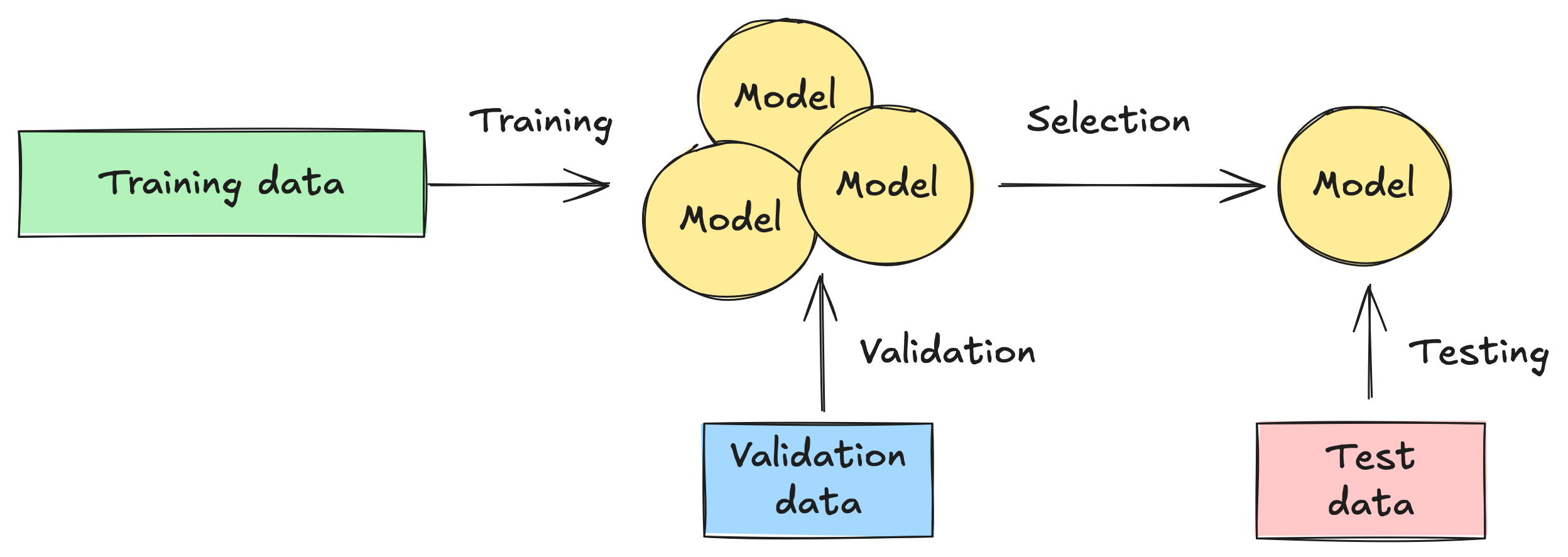
As with most problems in machine learning, the solution is more data—or rather, different data. Instead of splitting our data into training and test data, we split it into three parts: training, validation, and test data—say 50% for training and 25% for each of validation and test. We can then use the validation data for model selection as follows:

First, we train our candidate models—of different levels of complexity—on the training data.
Next, we run the trained models on the validation data to compare their performance, and we select the model which minimizes validation error.
Optionally, we can retrain the selected model on the combination of the training and validation data—this will likely improve its performance.
Finally, we run the selected model on the test data to evaluate its performance on new, previously unseen data.

Just as before, we need to be careful to prevent data leakage in this process. For example if our data has group structure and we plan to use our model on new groups in the wild, then our training, validation, and test data sets should respect this structure—no group should appear in more than one of the data sets. If there's no underlying structure in our data, it's a good idea to randomly shuffle it before splitting to avoid the possibility of accidental patterns.

The model selection process outlined above is straightforward, but it only works well if we have enough data. Because we're reducing the amount of data available for initial training by reserving some for validation, the models are likely to have higher variance. If data is more scarce, we need to find a more creative solution.

Cross-validation

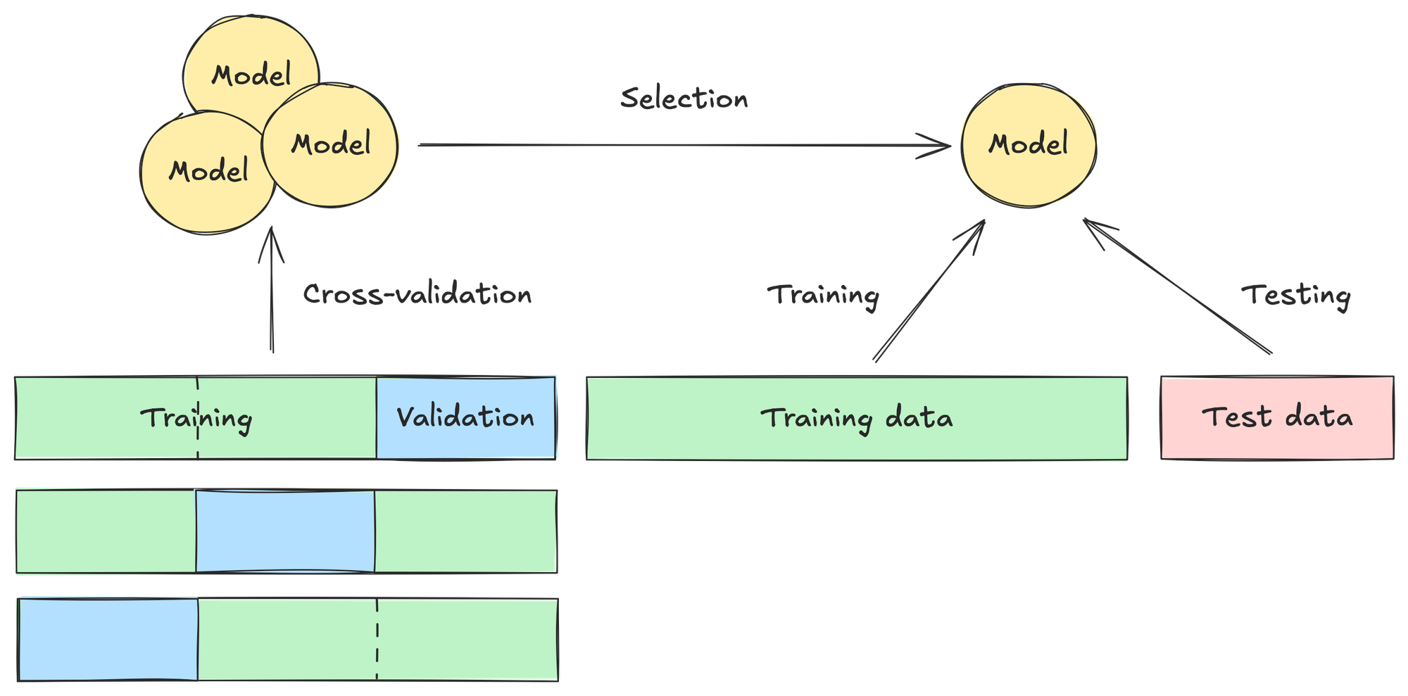
An alternative approach to model selection uses cross-validation, which makes more strategic use of the data we have available. It works as follows:

First we split our data into training and test data, as we did originally. But we now further split our training data into \(k\) parts called folds of roughly equal size—in practice, typically \(k=5\) or \(k=10\).
For each fold, we train the candidate models on the other \(k-1\) folds and validate the models on the current fold. This means that each model is validated \(k\) times, and has \(k\) validation error scores.
We average the \(k\) validation error scores for each model, and select the model with the lowest average score.
We retrain the selected model on all the training data.
Finally, we run the selected model on the test data to evaluate its performance.

Model selection with 3-fold cross-validation

Why is this process preferable to the previous one? For each fold, we're still reducing the amount of data available for training the models. However, by averaging the validation error scores over all the folds, we're helping to reduce variance in our error estimates—especially when we have more limited data available to start.

For a concrete example, suppose we have \(100\) samples in our full training data set. If we do \(5\)-fold cross-validation, then each fold's training subset will have \(80\) samples. Which samples appear in each subset is random—at least if we're shuffling before splitting. The subsets are similar to the full training set, but different enough from it—and from each other—that they have some degree of independence as training sets, so the resulting \(5\) validation error scores for each model also have some degree of independence. In general, taking an average—a mean—over independent outcomes of a random experiment reduces variance. This is the fundamental principle underlying the Law of Large Numbers in probability, and the reason why repeatedly flipping a coin gives us more information about whether it's fair.

What's critical to see is that the process of cross-validation gives us more information about how each type of model we're comparing—with its intrinsic level of complexity—performs on average when trained on data similar to the data it will ultimately be trained on. This helps us make a more balanced decision during model selection.

Bias and variance

The last point can be appreciated more fully by observing that there's a bias-variance tradeoff inherent in the very act of choosing the number of folds for cross-validation. Suppose we have \(n\) samples in our full training set, so the number \(k\) of folds satisfies \(2\le k\le n\).

At one extreme, we could choose \(k=2\), so that for each fold we have only about \(n/2\) samples available for training. This number is much smaller than \(n\), and a model trained on this many samples is likely to perform worse than it will when trained on \(n\) samples. In other words, we're introducing bias into our error estimate. At the same time, the model is more likely to learn too much about the particular samples in the smaller training subsets, resulting in higher variance. Since we're only averaging over two folds, we're not reducing that variance much.

At the other extreme, we could choose \(k=n\). This is known as leave-one-out cross-validation because with each fold we're leaving out one sample for validation while training on the other \(n-1\) samples. Since each training subset is almost the full training set, validation provides an almost unbiased estimate of error. However, all the training subsets are highly correlated with one other—they lack independence—so averaging over the folds may not reduce variance, even with \(n\) of them. It's important to see that this is true even though there's no longer any randomness as to which samples appear in each training subset—we're considering all possible subsets of \(n-1\) samples—so the error estimates will always be the same when we run cross-validation on the full training set.

The choice of \(k\) in a "sweet spot" between the extremes of \(2\) and \(n\) helps achieve a compromise between bias and variance in our error estimates. We saw an example with \(k=5\) above. With \(k=10\), each training subset contains about \(90\%\) of the full training set, which reduces bias but still yields enough independence that averaging over the \(10\) folds reduces variance. Once again, we see the importance of bias and variance in understanding and controlling error—but this time it's for error in error estimates.

Errors

We've seen that cross-validation allows us to estimate the error of a candidate model in a more balanced way. But exactly which error does cross-validation estimate, and is it the one we really want to estimate? Given the fact that we'll ultimately be training the selected model on the full training set, what we want to estimate is the error of a candidate model when it's trained on the full training set. To describe this precisely, we need a little bit of math.

Suppose our full training set is \[T=\{(\vec{x} _1, y _1),\ldots,(\vec{x} _n, y _n)\}\] where the \(\vec{x} _i\) are feature vectors and the \(y _i\) are corresponding target values. We can think of \(T\) as the result of randomly sampling \(n\) times from the population of all such pairs \((\vec{x},y)\) in the world. Equivalently, we can think of \(T\) itself as one possible value of the random training set \[\mathcal{T}=\{(\vec{X} _1, Y _1),\ldots,(\vec{X} _n, Y _n)\}\] with \(n\) independent random pairs \((\vec{X} _i, Y _i)\) following the population distribution. Here we distinguish notationally between a random variable like \(Y _i\)—a random quantity with a probability distribution—and a specific value of that variable like \(y _i\). The idea is that \(\mathcal{T}\) is a random variable while \(T\) is a specific value of that variable.

We can similarly think of a candidate model \(f\) trained on \(T\) as one possible value of a random model \(F\) trained on \(\mathcal{T}\)—that is, \(F=f\) when \(\mathcal{T}=T\). If \(E(F(\vec{X}), Y)\) denotes the error in the model prediction \(F(\vec{X})\) of the target \(Y\) for the pair \((\vec{X},Y)\), then the estimated model error conditional on the training set \(\mathcal{T}=T\) can be expressed as \[\mathbb{E} _{(\vec{X},Y)}[E(F(\vec{X}), Y)|\mathcal{T}=T]\] Here \(\mathbb{E} _{(\vec{X},Y)}\) denotes the expected value over the random pair \((\vec{X},Y)\) following the population distribution—intuitively, a weighted average where the weights are the probabilities of the pairs in the distribution.

This conditional estimated model error is what we're after, but it doesn't account for the randomness of the training set itself. For that, we can consider the unconditional estimated model error \[\mathbb{E} _{\mathcal{T}}[\mathbb{E} _{(\vec{X},Y)}[E(F(\vec{X}),Y)]]\] Here \(\mathbb{E} _{\mathcal{T}}\) averages over all possible training sets. This describes how the type of model will perform on average for new inputs from the population when trained on \(n\) independent samples from the population.

So, which type of error does cross-validation actually estimate? It turns out that it estimates the unconditional error better than the conditional error! From our observations earlier, this isn't totally surprising when the number of folds is in the "sweet spot", like \(k=5\) or \(k=10\). It's perhaps more surprising in the case of leave-one-out cross-validation when \(k=n\). But even in that case, empirical simulations show that the estimates from cross-validation better align with unconditional error estimates. Somewhat ironically, it's more difficult to estimate error conditional on the training set when all we have is the one training set! The good news is that unconditional error estimates—and likewise cross-validation error estimates—are still very useful for model selection, which was our original problem.