Beta-gammatene

One of the reasons that probability theory is so interesting—and challenging—is that simple questions can quickly lead to deep philosophical and mathematical issues. Suppose we have a coin and want to determine the probability of the coin landing heads when flipped. What does "probability" mean in this context? One thought is that the probability is something like the relative frequency of heads in repeated flips of the coin—if the coin lands heads a third of the time when flipped, then the probability of it landing heads when flipped is one third.

But which flips are we talking about here? Even if the coin is never actually flipped, it still has a probability of landing heads if it were to be flipped. The flips defining this probability must therefore be hypothetical. But which hypothetical flips? Intuitively, even if there's a nonzero likelihood of getting heads on a single flip, it's possible to get tails on every flip in a sequence of flips—even an infinite sequence, although the likelihood is vanishingly small. So the relative frequency in any particular sequence need not tell us the probability, and we need a way to understand the relative frequency in "most" or "almost all" sequences. The longer that such sequences are, the more information that they reveal about the probability, so we might as well take them all to be infinite. In these sequences, we also need to know that the outcome of one flip doesn't affect the outcome of another—in other words, that the flips are independent. We summarize the thought:

Frequency Thought: The probability of a coin landing heads when flipped is the limiting relative frequency of the coin landing heads in almost all infinite sequences of hypothetical independent flips.

It takes some work to realize the Frequency Thought in a mathematically rigorous way, but let's ignore that. Denote the probability by \(p\). Practically speaking, how do we actually compute \(p\)? On this view, we can only approximate it by computing relative frequencies of heads in finite sequences of actual independent flips. The more flips we do, the better our approximation becomes. But the true value of \(p\) is something that God only knows. Mathematically, \(p\) is treated as a fixed but unknown number between \(0\) and \(1\).

Even with its subtleties, this thought has intuitive appeal for random experiments like coin flips which can be repeated indefinitely. It's more awkward in other cases. For example, what's the probability that it will rain today? Whatever the value of that probability might be, it seems odd to think of it as the limiting relative frequency of rain in sequences of hypothetical occurrences of the day. Perhaps we could profitably consider sequences of days like today in relevant respects. Alternatively, we could think of the probability as our degree of belief or confidence in it raining today, given the information we have. We can also apply this thought to the coin:

Belief Thought: The probability of a coin landing heads on a given flip is a degree of belief in the coin landing heads on that flip.

Critically, whose degree of belief does this probability reflect? If it were God's, arguably the probability would either be \(0\) or \(1\) because God has no uncertainty about the outcome. If not God's, then whose? It seems problematic from a mathematical point of view that the probability should depend on the existence of an actual person forming an actual belief about the outcome, or that the value of the probability might vary depending on the person. We could develop a theory of hypothetical, idealized rational agents to try to solve this problem, but that would take work.

A more modest mathematical proposal along these lines is, rather than treating \(p\) as a fixed unknown number, to treat \(p\) as a random variable—that is, a random value between \(0\) and \(1\) which itself has a probability distribution. God only knows the actual distribution—possibly a point mass at a single value—but we can start with an initial assumption for a distribution and update it based on evidence we obtain from repeated independent coin flips. In some ways, we haven't changed anything under this proposal—we're still approximating an unknown through experiments. But a probability distribution can serve as a mathematical model of a degree of belief at a particular point in time, based on information available at that time, allowing us to realize the Belief Thought in a mathematically rigorous way.

Beta distribution

Let's see how this works. To start, we'll assume that any value of \(p\) between \(0\) and \(1\) is equally likely—that is, our initial or prior distribution for \(p\) is the uniform distribution on the interval \([0,1]\), with density function \(f=1_{[0,1]}\): \[f(p)=1_{[0,1]}(p)=\begin{cases}1&\text{if }0\le p\le 1\\0&\text{otherwise}\end{cases}\] If we now flip the coin \(n\) times independently to obtain the outcomes \(x_1,\ldots,x_n\in\{0,1\}\)—where \(x_i=1\) if we obtain heads, and \(x_i=0\) if we obtain tails, on the \(i\)-th flip—then we can compute the posterior density function \(f(p|\vec{x})\) describing the updated probability distribution for \(p\) given the outcomes \(\vec{x}=(x_1,\ldots,x_n)\). From Bayes' Theorem, we know \[f(p|\vec{x})\propto f(\vec{x}|p)f(p)\] Here \(f(\vec{x}|p)\) is called the likelihood function for the outcomes \(\vec{x}\) given the probability \(p\). It gives the probability of observing the outcomes \(\vec{x}\) assuming that the probability of heads is \(p\). Since the flips are independent, we have \[f(\vec{x}|p)=\prod_{i=1} ^nf(x_i|p)\] We can cleverly write \(f(x_i|p)=p ^{x_i}(1-p) ^{1-x_i}\) with the convention that \(0 ^0=1\) to obtain \[f(\vec{x}|p)= p ^h(1-p) ^{n-h}\] where \(h=\sum_{i=1} ^n x_i\) is the number of heads and \(n-h\) is the number of tails among the outcomes \(\vec{x}\). It follows that \[f(p|\vec{x})\propto p ^h(1-p) ^{n-h}\quad(0\le p\le 1)\] and \(f(p|\vec{x})=0\) for other values of \(p\). Since \(f(p|\vec{x})\) is a density function, it must satisfy \[\int_0 ^1 f(p|\vec{x})\,dp=\int_{-\infty} ^{\infty}f(p|\vec{x})\,dp=1\] Using this to solve for the proportionality constant, we obtain \[f(p|\vec{x})=\frac{p ^h(1-p) ^{n-h}}{\int_0 ^1 p ^h(1-p) ^{n-h}\,dp}\quad(0<p<1)\] That integral in the denominator is important enough to deserve a name. We define the beta function \[\Beta(x,y)=\int_0 ^1 t ^{x-1}(1-t) ^{y-1}\,dt\quad(x,y>0)\] This integral exists for all \(x>0\) and \(y>0\) since \(t ^{x-1}(1-t) ^{y-1}\sim t ^{x-1}\) as \(t\to 0 ^+\) and \(x-1>-1\), and similar reasoning applies as \(t\to 1 ^-\). Using this function, we obtain \[\boxed{f(p|\vec{x})=\frac{p ^h(1-p) ^{n-h}}{\Beta(h+1,n-h+1)}\quad(0<p<1)}\] In words: given the outcomes of a finite sequence of independent flips of a coin, the probability of the coin landing heads when flipped follows a beta distribution with parameters given by—essentially—the number of heads and the number of tails in the outcomes. This distribution can serve to model our degree of belief about getting heads when we flip the coin.

Example: if we flip the coin \(10\) times and get \(3\) heads, then the density looks like this:

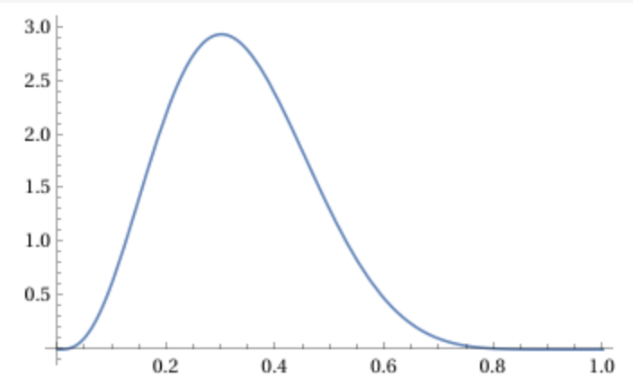
Notice how the mass—the area under the curve—is concentrated roughly around \(p=0.3\), which suggests that the probability of heads is around \(p=0.3=\frac{3}{10}\). Actually, the mean of the posterior distribution is \(\overline{p}=\frac{1}{3}\), which is a weighted average of \(\frac{3}{10}\) and the prior mean \(\frac{1}{2}\). The more flips we do, the tighter the distribution becomes concentrated around the posterior mean determined by the observed outcomes.

Beta function

The beta function has a number of useful properties. Substituting \(s=1-t\) in the defining integral, we obtain \[\Beta(x,y)=\Beta(y,x)\] showing that the beta function is symmetric. Rewriting the integral and integrating by parts, we obtain the recursion formula \[\begin{align}\Beta(x+1,y)&=\int_0 ^1\Bigl(\frac{t}{1-t}\Bigr) ^x(1-t) ^{x+y-1}\,dt\notag\\&=-\Bigl(\frac{t}{1-t}\Bigr) ^x\frac{(1-t) ^{x+y}}{x+y}\biggl.\biggr|_0 ^1+\frac{x}{x+y}\int _0 ^1(1-t) ^{x+y}\Bigl(\frac{t}{1-t}\Bigr) ^{x-1}\frac{dt}{(1-t) ^2}\notag\\&=\frac{x}{x+y}\Beta(x,y)\notag\end{align}\] It follows that \[\Beta(x,n+1)=\Beta(n+1,x)=\frac{n}{n+x}\Beta(n,x)=\frac{n}{x+n}\Beta(x,n)\] Since \(\Beta(x,1)=\frac{1}{x}\), it follows by induction on \(n\) that \[\Beta(x,n+1)=\frac{n!}{x(x+1)\cdots(x+n)}\] On the other hand, substituting \(s=nt\) into the defining integral, we obtain \[\Beta(x,n+1)=n ^{-x}\int _0 ^n s ^{x-1}\Bigl(1-\frac{s}{n}\Bigr) ^n\,ds\] Since \[\lim _{n\to\infty}\Bigl(1-\frac{s}{n}\Bigr) ^n=e ^{-s}\] it can be shown that \[\lim _{n\to\infty}\int _0 ^n s ^{x-1}\Bigl(1-\frac{s}{n}\Bigr) ^n\,ds=\int _0 ^{\infty}s ^{x-1}e ^{-s}\,ds\] The integral on the right, which exists for all \(x>0\), is another extremely important function in mathematics called the gamma function: \[\Gamma(x)=\int _0 ^{\infty}t ^{x-1}e ^{-t}\,dt\quad(x>0)\] From the above we have \[\Gamma(x)=\lim _{n\to\infty}n ^x\,\Beta(x,n+1)\] and hence \[\boxed{\Gamma(x)=\lim _{n\to\infty}\frac{n ^xn!}{x(x+1)\cdots(x+n)}}\] This formula was first discovered by Euler or Gauss, depending on who you ask. Both the beta and gamma integrals were studied by Euler.

Gamma function

While we're here, let's take a closer look at the gamma function. It's immediate that \(\Gamma(1)=1\), and it follows from the recursion formula for the beta function that the gamma function satisfies the recursion formula \[\Gamma(x+1)=x\Gamma(x)\] In particular \[\Gamma(n+1)=n!\] which shows that the gamma function generalizes the factorial function from the positive integers to the positive reals. In fact, the gamma function is the only function satisfying these properties which is log convex—meaning that \(\log\Gamma(x)\) is convex.

We can exploit the latter universal property to prove things without getting our hands too dirty. As an example, for fixed \(y>0\) consider the function \[g(x)=\Beta(x,y)\frac{\Gamma(x+y)}{\Gamma(y)}\quad(x>0)\] It's easy to see that \(g(1)=1\) and \(g(x+1)=xg(x)\). Since \(g\) is a product of two log convex functions, it's log convex. Therefore \(g(x)=\Gamma(x)\) and hence \[\boxed{\Beta(x,y)=\frac{\Gamma(x)\Gamma(y)}{\Gamma(x+y)}}\] Taking \(x=y=\frac{1}{2}\) and making the substitution \(t=\sin ^2\varphi\) in the integral for the beta function, we obtain \[\Gamma(\tfrac{1}{2})=\sqrt{\pi}\] which is useful in the computation of certain integrals.

Gamma distribution

Returning to probability theory, the gamma function itself makes an appearance in an important distribution called—surprisingly enough—the gamma distribution, which has density \[f(x)=\frac{x ^{\alpha-1}e ^{-x}}{\Gamma(\alpha)}\quad(x>0)\] Here \(\alpha>0\) is a parameter controlling the shape of the distribution.

Example: For \(\alpha=2\) the density \(f(x)=xe ^{-x}\) looks like this:

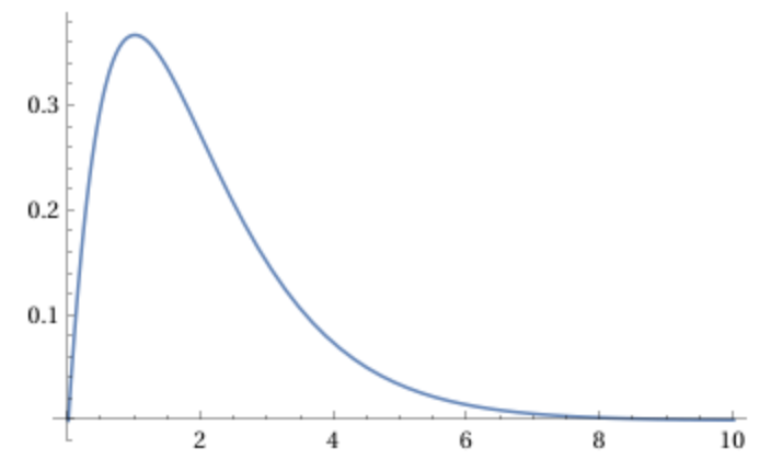
This shape is intuitive. We have \(f(0)=0\) and \(f(x)>0\) for \(x>0\). Since \(e ^{-x}\to 0\) faster than \(x\to\infty\) as \(x\to\infty\), it follows that \(xe ^{-x}\to 0\) as \(x\to\infty\). Since \[f'(x)=e ^{-x}-xe ^{-x}=(1-x)e ^{-x}=0\] only when \(x=1\), it follows that \(f\) attains its maximum at \(x=1\). In general, the gamma density with parameter \(\alpha>1\) attains its maximum at \(x=\alpha-1\). This type of gamma distribution is commonly used to model waiting times.

Conclusion

We see that the realization of the Belief Thought not only provides a rigorous and powerful framework for probability, but also leads to some very interesting mathematics. Starting from a simple question about flipping a coin, we quickly find ourselves hobnobbing with Euler, Gauss, and other great minds. This is part of the pleasure of probability theory!